Exploratory Data Analysis (EDA) and Statistical Analysis in R Programming

In this project, I worked with a large dataset about US traffic accidents. I've applied exploratory data analysis followed by a statistical investigation of various aspects of the data. This large dataset was cleaned, analyzed and visualized in R Programming.

Initially, the data was imported into the R environment, followed by a preliminary examination of the structure and properties of the data. This involved looking at the various columns in the dataset, understanding the types of data (numerical, categorical, date/time), and recognizing the presence of missing values.

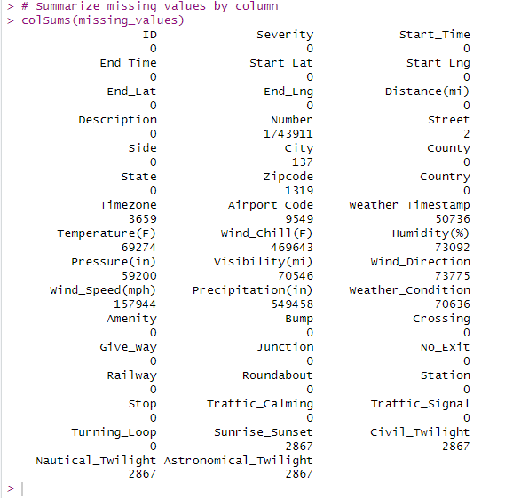
Upload the data and examine missing values.

library(readr)

#Upload the dataset

US_accidents <- read_csv("R project/US_Accidents_Dec21_updated.csv")

#Data structure

str(US_accidents)

#Identifying missing values

missing_values <- is.na(US_accidents)

# Summarize missing values by column

colSums(missing_values)

OUTPUT:

Data cleaning was then performed to handle missing values, with numerical missing values replaced by mean values, and categorical missing values replaced by 'NULL'.

# Copy of the dataset to not modify the original data

US_accidents_clean <- US_accidents

****Replace numerical columns with the median of their respective columns****

# Replace missing values in 'Temperature(F)' with its median

US_accidents_clean$`Temperature(F)`[is.na(US_accidents_clean$`Temperature(F)`)] <- median(US_accidents_clean$`Temperature(F)`, na.rm = TRUE)

# Replace missing values in 'Wind_Chill(F)' with its median

US_accidents_clean$`Wind_Chill(F)`[is.na(US_accidents_clean$`Wind_Chill(F)`)] <- median(US_accidents_clean$`Wind_Chill(F)`, na.rm = TRUE)

# Replace missing values in 'Humidity(%)' with its median

US_accidents_clean$`Humidity(%)`[is.na(US_accidents_clean$`Humidity(%)`)] <- median(US_accidents_clean$`Humidity(%)`, na.rm = TRUE)

# Replace missing values in 'Pressure(in)' with its median

US_accidents_clean$`Pressure(in)`[is.na(US_accidents_clean$`Pressure(in)`)] <- median(US_accidents_clean$`Pressure(in)`, na.rm = TRUE)

# Replace missing values in 'Visibility(mi)' with its median

US_accidents_clean$`Visibility(mi)`[is.na(US_accidents_clean$`Visibility(mi)`)] <- median(US_accidents_clean$`Visibility(mi)`, na.rm = TRUE)

# Replace missing values in 'Wind_Speed(mph)' with its median

US_accidents_clean$`Wind_Speed(mph)`[is.na(US_accidents_clean$`Wind_Speed(mph)`)] <- median(US_accidents_clean$`Wind_Speed(mph)`, na.rm = TRUE)

# Replace missing values in 'Precipitation(in)' with its median

US_accidents_clean$`Precipitation(in)`[is.na(US_accidents_clean$`Precipitation(in)`)] <- median(US_accidents_clean$`Precipitation(in)`, na.rm = TRUE)

****Replace categorical columns with 'NULL****

# Replace missing values in 'Number' with 'NULL'

US_accidents_clean$Number[is.na(US_accidents_clean$Number)] <- 'NULL'

# Replace missing values in 'City' with 'NULL'

US_accidents_clean$City[is.na(US_accidents_clean$City)] <- 'NULL'

# Replace missing values in 'Zipcode' with 'NULL'

US_accidents_clean$Zipcode[is.na(US_accidents_clean$Zipcode)] <- 'NULL'

# Replace missing values in 'Timezone' with 'NULL'

US_accidents_clean$Timezone[is.na(US_accidents_clean$Timezone)] <- 'NULL'

# Replace missing values in 'Airport_Code' with 'NULL'

US_accidents_clean$Airport_Code[is.na(US_accidents_clean$Airport_Code)] <- 'NULL'

# Replace missing values in 'Weather_Timestamp' with 'NULL'

US_accidents_clean$Weather_Timestamp[is.na(US_accidents_clean$Weather_Timestamp)] <- NA

# Replace missing values in 'Wind_Direction' with 'NULL'

US_accidents_clean$Wind_Direction[is.na(US_accidents_clean$Wind_Direction)] <- 'NULL'

# Replace missing values in 'Weather_Condition' with 'NULL'

US_accidents_clean$Weather_Condition[is.na(US_accidents_clean$Weather_Condition)] <- 'NULL'

# Replace missing values in 'Sunrise_Sunset' with 'NULL'

US_accidents_clean$Sunrise_Sunset[is.na(US_accidents_clean$Sunrise_Sunset)] <- 'NULL'

# Replace missing values in 'Civil_Twilight' with 'NULL'

US_accidents_clean$Civil_Twilight[is.na(US_accidents_clean$Civil_Twilight)] <- 'NULL'

# Replace missing values in 'Nautical_Twilight' with 'NULL'

US_accidents_clean$Nautical_Twilight[is.na(US_accidents_clean$Nautical_Twilight)] <- 'NULL'

# Replace missing values in 'Astronomical_Twilight' with 'NULL'

US_accidents_clean$Astronomical_Twilight[is.na(US_accidents_clean$Astronomical_Twilight)] <- 'NULL'

#*****Explore and analyze the new dataset

#Structure of the new data

str(US_accidents_clean)

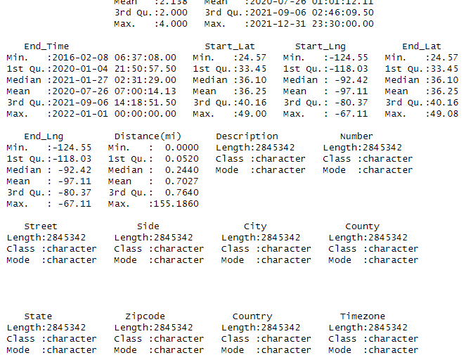
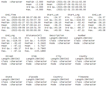
#Summary of the new data

summary(US_accidents_clean

OUTPUT:

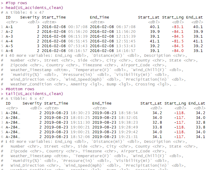
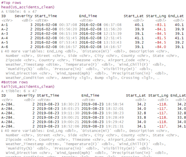
#Top rows

head(US_accidents_clean)

#Bottom rows

tail(US_accidents_clean)

OUTPUT:

#Check for missing values again

colSums(is.na(US_accidents_clean))

OUTPUT:

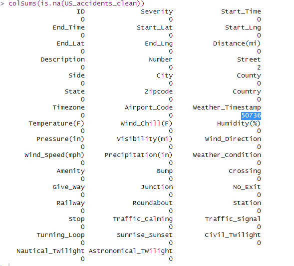
Note: weather_Timestamp shows 50736 missing values, When I replaced the missing values in 'Weather_Timestamp' with NA, I was essentially replacing NA with NA. This means I haven't actually changed anything, so when I run colSums(is.na()) again, it will still show the same number of missing values.

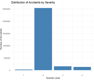
****distribution of accidents based on the 'Severity' level.****

install.packages("ggplot2")

library(ggplot2)

ggplot(US_accidents_clean, aes(x = Severity)) +

geom_bar(fill = "steelblue") +

theme_minimal() +

labs(title = "Distribution of Accidents by Severity", x = "Severity Level", y = "Number of Accidents")

PLOT:

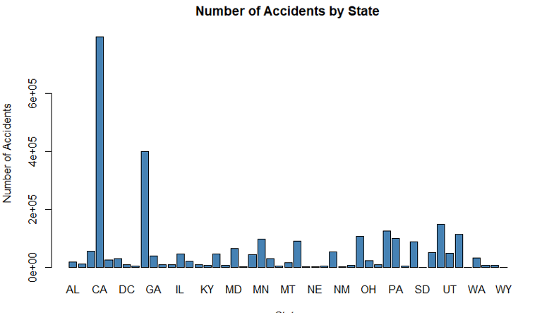
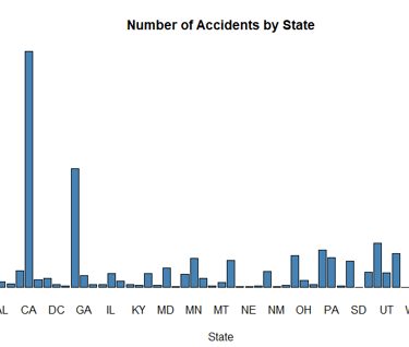
*****Find out the most accident-prone states.*****

state_counts <- table(US_accidents_clean$State)

barplot(state_counts, main="Number of Accidents by State", xlab="State", ylab="Number of Accidents", col="steelblue")

PLOT:

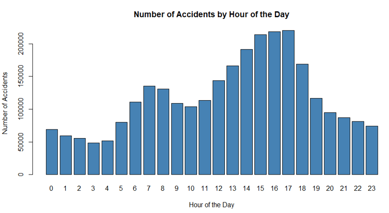
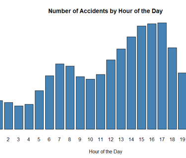
*****Analyze the trend of accidents over time.****

# Convert the 'Start_Time' column to a POSIXlt object

US_accidents_clean$Start_Time <- as.POSIXlt(US_accidents_clean$Start_Time)

# Extract the hour from the 'Start_Time' column

US_accidents_clean$Hour <- US_accidents_clean$Start_Time$hour

# Get the count of accidents for each hour

hour_counts <- table(US_accidents_clean$Hour)

# Plot the data

barplot(hour_counts, main="Number of Accidents by Hour of the Day", xlab="Hour of the Day", ylab="Number of Accidents", col="steelblue")

PLOT:

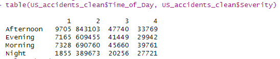
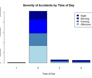
*****examine if the time of day affects the severity of accidents.****

#Create the variable "Hour" as a column

US_accidents_clean$Start_Time <- as.POSIXct(US_accidents_clean$Start_Time)

US_accidents_clean$hour <- format(US_accidents_clean$Start_Time, format = "%H")

US_accidents_clean$hour <- as.numeric(US_accidents_clean$hour)

#Classify each accident into a time period

US_accidents_clean$Time_of_Day[US_accidents_clean$hour >= 5 & US_accidents_clean$hour < 12] <- 'Morning'

US_accidents_clean$Time_of_Day[US_accidents_clean$hour >= 12 & US_accidents_clean$hour < 17] <- 'Afternoon'

US_accidents_clean$Time_of_Day[US_accidents_clean$hour >= 17 & US_accidents_clean$hour < 22] <- 'Evening'

US_accidents_clean$Time_of_Day[US_accidents_clean$hour >= 22 | US_accidents_clean$hour < 5] <- 'Night'

table(US_accidents_clean$Time_of_Day, US_accidents_clean$Severity)

OUTPUT:

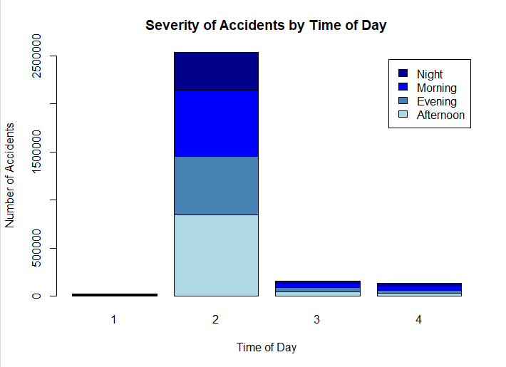
#plot the data

severity_time_of_day <- table(US_accidents_clean$Time_of_Day, US_accidents_clean$Severity)

barplot(severity_time_of_day,

main = "Severity of Accidents by Time of Day",

xlab = "Time of Day",

ylab = "Number of Accidents",

col = c("lightblue", "steelblue", "blue", "darkblue"),

legend = rownames(severity_time_of_day))

PLOT:

If we are interested in Investigating if certain weather conditions contribute to a higher number of accidents

weather_counts <- table(US_accidents_clean$Weather_Condition)

# Sort the counts in descending order

sorted_weather <- sort(weather_counts, decreasing = TRUE)

# Print the results

print(sorted_weather)

Note: Running the provided codes will generate a list that represents the total count of traffic accidents categorized by different weather conditions.

Back to projects